Simulation using Karhunen-Loève decomposition

# Author: Steven Golovkine <steven_golovkine@icloud.com>
# License: MIT

# Load packages
import numpy as np

from FDApy.representation import DenseArgvals
from FDApy.simulation import KarhunenLoeve
from FDApy.visualization import plot

The simulation of univariate functional data \(X: \mathcal{T} \rightarrow \mathbb{R}\) is based on the truncated Karhunen-Loève representation of \(X\). Consider that the representation is truncated at \(K\) components, then, for a particular realization \(i\) of the process \(X\):

\[X_i(t) = \mu(t) + \sum_{k = 1}^K c_{i, k}\phi_k(t), \quad t \in \mathcal{T}\]

with a common mean function \(\mu(t)\) and eigenfunctions \(\phi_k, k = 1, \cdots, K\). The scores \(c_{i, k}\) are the projection of the curves \(X_i\) onto the eigenfunctions \(\phi_k\). These scores are random variables with mean \(0\) and variance \(\lambda_k\), which are the eigenvalues associated to each eigenfunctions and that decreases toward \(0\) when \(k\) goes to infinity. This representation is valid for domains of arbitrary dimension, such as images (\(\mathcal{T} = \mathbb{R}^2\)).

# Set general parameters
rng = 42
n_obs = 10

# Parameters of the basis
name = "fourier"
n_functions = 25
argvals = DenseArgvals({"input_dim_0": np.arange(0, 10.01, 0.01)})

Simulation for one-dimensional curve

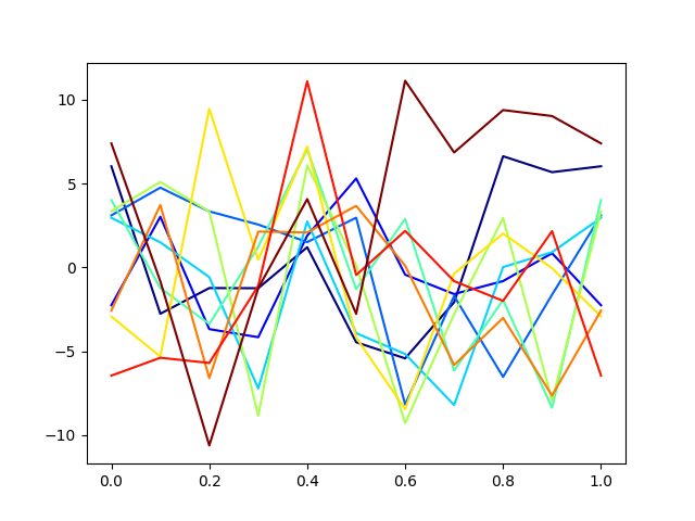
First example — We simulate \(N = 10\) curves on the one-dimensional observation grid \(\{0, 0.1, 0.2, \cdots, 1\}\) (default), based on the first \(K = 25\) Fourier basis functions on \([0, 1]\) and the variance of the scores random variables equal to \(1\) (default).

kl = KarhunenLoeve(
    basis_name=name, n_functions=n_functions, random_state=rng
)
kl.new(n_obs=n_obs)

_ = plot(kl.data)

Second example — We simulate \(N = 10\) curves on the one-dimensional observation grid \(\{0, 0.01, 0.02, \cdots, 10\}\), based on the first \(K = 25\) Fourier basis functions on \([0, 10]\) and the variance of the scores random variables equal to \(1\) (default).

kl = KarhunenLoeve(
    basis_name=name, argvals=argvals, n_functions=n_functions, random_state=rng
)
kl.new(n_obs=n_obs)

_ = plot(kl.data)

Third example — We simulate \(N = 10\) curves on the one-dimensional observation grid \(\{0, 0.01, 0.02, \cdots, 10\}\) (default), based on the first \(K = 25\) Fourier basis functions on \([0, 1]\) and the decreasing of the variance of the scores is exponential.

kl = KarhunenLoeve(
    basis_name=name, argvals=argvals, n_functions=n_functions, random_state=rng
)
kl.new(n_obs=n_obs, clusters_std="exponential")

_ = plot(kl.data)

Simulation for two-dimensional curve (image)

For the simulation on a two-dimensional domain, we construct an two-dimensional eigenbasis based on tensor products of univariate eigenbasis.

First example — We simulate \(N = 1\) image on the two-dimensional observation grid \(\{0, 0.01, 0.02, \cdots, 10\} \times \{0, 0.01, 0.02, \cdots, 10\}\) (default), based on the tensor product of the first \(K = 25\) Fourier basis functions on \([0, 10] \times [0, 10]\) and the variance of the scores random variables equal to \(1\) (default).

# Parameters of the basis
name = ("fourier", "fourier")
n_functions = (5, 5)
argvals = DenseArgvals(
    {"input_dim_0": np.arange(0, 10.01, 0.01), "input_dim_1": np.arange(0, 10.01, 0.01)}
)

kl = KarhunenLoeve(
    basis_name=name, argvals=argvals, n_functions=n_functions, random_state=rng
)
kl.new(n_obs=1)

_ = plot(kl.data)

Second example — We simulate \(N = 1\) image on the two-dimensional observation grid \(\{0, 0.01, 0.02, \cdots, 1\} \times \{0, 0.01, 0.02, \cdots, 1\}\) (default), based on the tensor product of the first \(K = 25\) Fourier basis functions on \([0, 1] \times [0, 1]\) and the decreasing of the variance of the scores is linear.

kl = KarhunenLoeve(
    basis_name=name, argvals=argvals, n_functions=n_functions, random_state=rng
)
kl.new(n_obs=1, clusters_std="linear")

_ = plot(kl.data)