FPCA of 2-dimensional data

# Author: Steven Golovkine <steven_golovkine@icloud.com>
# License: MIT

# Load packages
import matplotlib.pyplot as plt
import numpy as np

from FDApy.representation import DenseArgvals
from FDApy.simulation import KarhunenLoeve
from FDApy.preprocessing import UFPCA, FCPTPA
from FDApy.visualization import plot

In this section, we are showing how to perform a functional principal component on two-dimensional data using the UFPCA and FCPTPA classes. We will compare two methods to perform the dimension reduction: the FCP-TPA and the decomposition of the inner-product matrix. We will use the first \(K = 5\) principal components to reconstruct the curves.

# Set general parameters
rng = 42
n_obs = 50

# Parameters of the basis
name = ("fourier", "fourier")
n_functions = (5, 5)
argvals = DenseArgvals({
    "input_dim_0": np.linspace(0, 1, 21),
    "input_dim_1": np.linspace(-0.5, 0.5, 21)
})

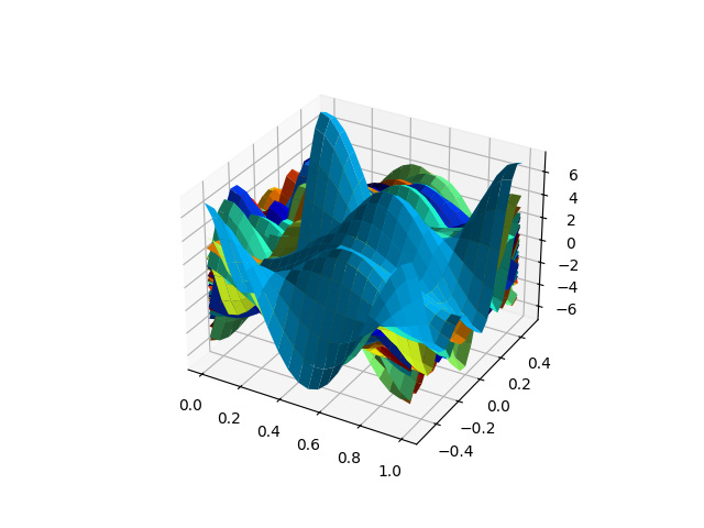
We simulate \(N = 50\) images on the two-dimensional observation grid \(\{0, 0.05, 0.1, \cdots, 1\} \times \{0, 0.05, 0.1, \cdots, 1\}\), based on the tensor product of the first \(K = 5\) Fourier basis functions on \([0, 1] \times [0, 1]\) and the variance of the scores random variables decreases exponentially.

kl = KarhunenLoeve(
    basis_name=name,
    n_functions=n_functions,
    argvals=argvals,
    add_intercept=False,
    random_state=rng,
)
kl.new(n_obs=n_obs, clusters_std="exponential")
data = kl.data

_ = plot(data)

Estimation of the eigencomponents

The class FCPTPA requires two parameters: the number of components to estimate and if normalization is needed. The method also requires hyperparameters for the FCP-TPA algorithm. The hyperparameters are the penalty matrices for the first and second dimensions, the range of the alpha parameter for the first and second dimensions, the tolerance for the convergence of the algorithm, the maximum number of iterations, and if the tolerance should be adapted during the iterations. The class UFPCA requires two parameters: the number of components to estimate and the method to use. For two-dimensional data, the method parameter can only be inner-product. It will estimate the eigenfunctions by decomposing the inner-product matrix.

# First, we perform a univariate FPCA using the FPCTPA.
# Hyperparameters for FCP-TPA
n_points = data.n_points
mat_v = np.diff(np.identity(n_points[0]))
mat_w = np.diff(np.identity(n_points[1]))

penal_v = np.dot(mat_v, mat_v.T)
penal_w = np.dot(mat_w, mat_w.T)

ufpca_fcptpa = FCPTPA(n_components=5, normalize=True)
ufpca_fcptpa.fit(
    data,
    penalty_matrices={"v": penal_v, "w": penal_w},
    alpha_range={"v": (1e-4, 1e4), "w": (1e-4, 1e4)},
    tolerance=1e-4,
    max_iteration=15,
    adapt_tolerance=True,
)

# Second, we perform a univariate FPCA using a decomposition of the inner-product matrix.
ufpca_innpro = UFPCA(n_components=5, method="inner-product")
ufpca_innpro.fit(data)

/home/docs/checkouts/readthedocs.org/user_builds/fdapy/envs/latest/lib/python3.10/site-packages/FDApy/preprocessing/dim_reduction/ufpca.py:572: UserWarning: The estimation of the covariance is not performed for 2-dimensional data.
  warnings.warn(

Estimation of the scores

Once the eigenfunctions are estimated, we can estimate the scores – projection of the curves onto the eigenfunctions – using the eigenvectors from the decomposition of the covariance operator or the inner-product matrix. We can then reconstruct the curves using the scores. The transform() method requires the data as argument and the method to use. The method parameter can be either NumInt, PACE or InnPro. Note that, when using the eigenvectors from the decomposition of the inner-product matrix, new data can not be passed as argument of the transform method because the estimation is performed using the eigenvectors of the inner-product matrix.

scores_fcptpa = ufpca_fcptpa.transform(data)
scores_innpro = ufpca_innpro.transform(method="InnPro")

# Plot of the scores
plt.scatter(scores_fcptpa[:, 0], scores_fcptpa[:, 1], label="FCPTPA")
plt.scatter(scores_innpro[:, 0], scores_innpro[:, 1], label="InnPro")
plt.legend()
plt.show()

Comparison of the methods

Finally, we compare the methods by reconstructing the curves using the first \(K = 5\) principal components. We plot a sample of curves and their reconstruction.

data_recons_fcptpa = ufpca_fcptpa.inverse_transform(scores_fcptpa)
data_recons_innpro = ufpca_innpro.inverse_transform(scores_innpro)

fig, axes = plt.subplots(nrows=5, ncols=3, figsize=(16, 16))
for idx_plot, idx in enumerate(np.random.choice(n_obs, 5)):
    axes[idx_plot, 0] = plot(data[idx], ax=axes[idx_plot, 0])
    axes[idx_plot, 0].set_title("True")

    axes[idx_plot, 1] = plot(data_recons_fcptpa[idx], ax=axes[idx_plot, 1])
    axes[idx_plot, 1].set_title("FCPTPA")

    axes[idx_plot, 2] = plot(data_recons_innpro[idx], ax=axes[idx_plot, 2])
    axes[idx_plot, 2].set_title("InnPro")
plt.show()