One-dimensional Basis

# Author: Steven Golovkine <steven_golovkine@icloud.com>
# License: MIT

# Load packages
import numpy as np

from FDApy.representation import Basis
from FDApy.representation import DenseArgvals
from FDApy.visualization import plot

The package include different basis functions to represent functional data. In this section, we are showing the building blocks of the representation of basis functions. To define a Basis object, we need to specify the name of the basis, the number of functions in the basis and the sampling points. The sampling points are defined as a DenseArgvals.

We will show the basis functions for the Fourier, B-splines and Wiener basis. The number of functions in the basis is set to \(5\) and the sampling points are defined as a DenseArgvals object with a hundred points between \(0\) and \(1\).

# Parameters
n_functions = 5
argvals = DenseArgvals({"input_dim_0": np.linspace(0, 1, 101)})

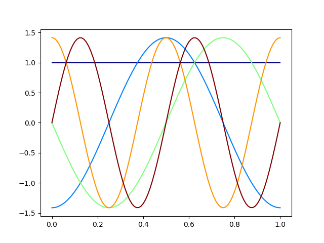
Fourier basis

First, we will show the basis functions for the Fourier basis. The basis functions consist of the sine and cosine functions with a frequency that increases with the number of the function. Note that the first function is a constant function. This basis may be used to represent periodic functions.

basis = Basis(name="fourier", n_functions=n_functions, argvals=argvals)

_ = plot(basis)

B-splines basis

Second, we will show the basis functions for the B-splines basis. The basis functions are piecewise polynomials that are smooth at the knots. The number of knots is equal to the number of functions in the basis minus \(2\). This basis may be used to represent smooth functions.

basis = Basis(name="bsplines", n_functions=n_functions, argvals=argvals)

_ = plot(basis)

Wiener basis

Third, we will show the basis functions for the Wiener basis. The basis functions are the eigenfunctions of a Brownian process. This basis may be used to represent rough functions.

basis = Basis(name="wiener", n_functions=n_functions, argvals=argvals)

_ = plot(basis)