Canadian weather dataset

# Author: Steven Golovkine <steven_golovkine@icloud.com>
# License: MIT

# Load packages
import matplotlib.pyplot as plt
import numpy as np

from FDApy.representation import DenseArgvals
from FDApy.preprocessing import UFPCA

from FDApy import read_csv
from FDApy.visualization import plot

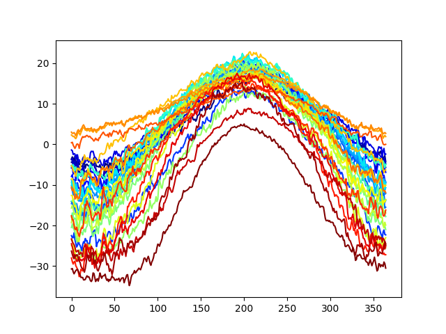
In this section, we will use the Canadian weather dataset to illustrate the use of the package. We will first load the data and plot it. Then, we will smooth the data using local polynomial regression. Finally, we will perform UFPCA on the smoothed data and plot the eigenfunctions.

First, we load the data. The dataset contains daily temperature data for \(35\) Canadian cities. The dataset can be downloaded from the here. This is an example of a DenseFunctionalData object. It also shows how the CSV file should be formatted and can be read using the read_csv() function.

# Load data
temp_data = read_csv("../data/canadian_temperature_daily.csv", index_col=0)

_ = plot(temp_data)
plt.show()

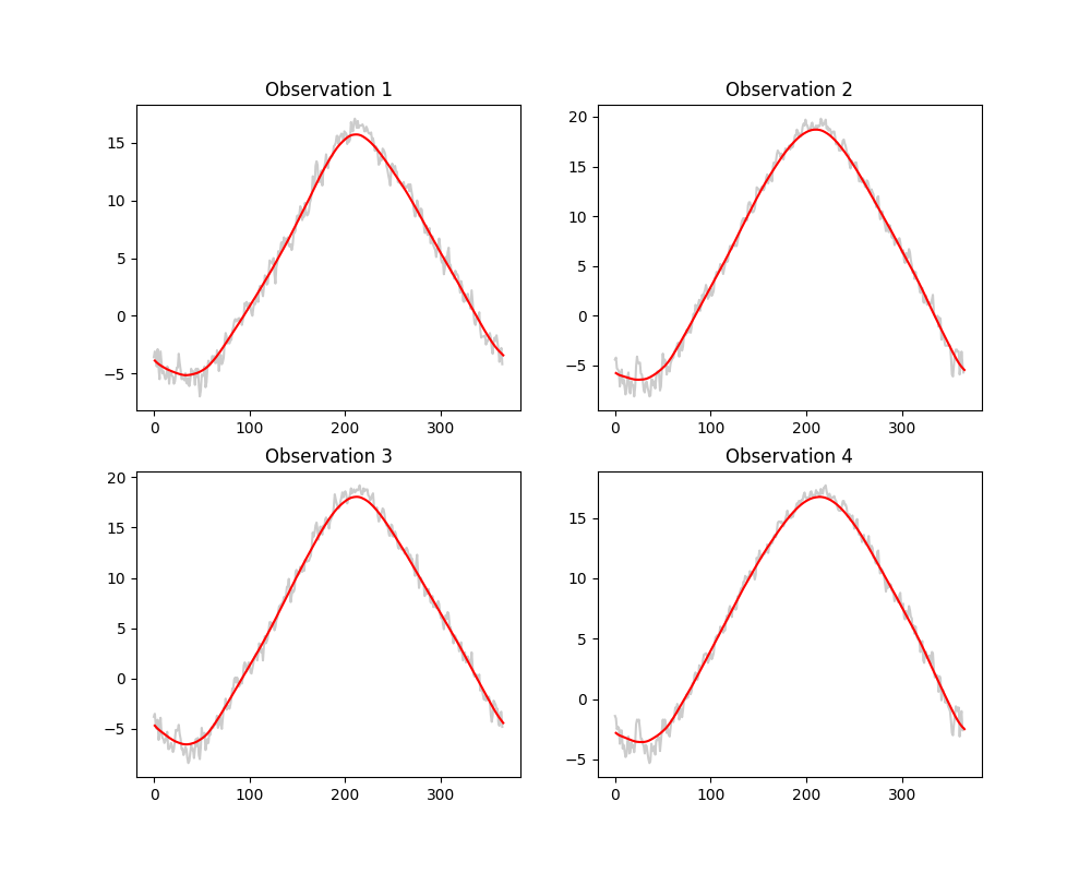
We will now smooth the data using local polynomial regression on the grid \(\{1, 2, 3, \dots, 365\}\). We will use the Epanechnikov kernel with a bandwidth of \(30\) and a degree of \(1\). The smoothing is performed using the smooth() method. We will then plot the smoothed data.

points = DenseArgvals({"input_dim_0": np.linspace(1, 365, 365)})
kernel_name = "epanechnikov"
bandwidth = 30
degree = 1

temp_smooth = temp_data.smooth(
    points=points,
    method="LP",
    kernel_name=kernel_name,
    bandwidth=bandwidth,
    degree=degree,
)

fig, axes = plt.subplots(2, 2, figsize=(10, 8))
for idx, ax in enumerate(axes.flat):
    plot(temp_data[idx], colors="k", alpha=0.2, ax=ax)
    plot(temp_smooth[idx], colors="r", ax=ax)
    ax.set_title(f"Observation {idx + 1}")
plt.show()

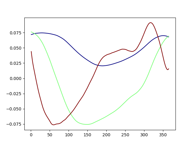
We will now perform UFPCA on the smoothed data. We will use the inner product method and keep the principal components that explain 99% of the variance. We will then plot the eigenfunctions. The scores are then computed using the inner-product matrix.

ufpca = UFPCA(n_components=0.99, method="inner-product")
ufpca.fit(temp_smooth)
scores = ufpca.transform(method="InnPro")

_ = plot(ufpca.eigenfunctions)
plt.show()

Finally, the data can be reconstructed using the scores. We plot the reconstruction of the first 10 observations.

data_recons = ufpca.inverse_transform(scores)

fig, axes = plt.subplots(nrows=5, ncols=2, figsize=(16, 16))
for idx_plot, idx in enumerate(np.random.choice(temp_data.n_obs, 10)):
    temp_ax = axes.flatten()[idx_plot]
    temp_ax = plot(temp_data[idx], colors="k", alpha=0.2, ax=temp_ax, label="Data")
    plot(temp_smooth[idx], colors="r", ax=temp_ax, label="Smooth")
    plot(data_recons[idx], colors="b", ax=temp_ax, label="Reconstruction")
    temp_ax.legend()
plt.show()