LocalPolynomial#
- class FDApy.preprocessing.LocalPolynomial(kernel_name='epanechnikov', bandwidth=0.05, degree=1, robust=False, **kwargs)[source]#
Local Polynomial regression.
This module implements Local Polynomial Regression over different dimensional domain [2]. The idea of local regression is to fit a (simple) different model separetely at each query point \(x_0\). Using only the observations close to \(x_0\), the resulting estimated function is smooth in the definition domain. Selecting observations close to \(x_0\) is achieved via a weighted (kernel) function which assigned a weight to each observation based on its (euclidean) distance from the query point.
Different kernels are defined (gaussian, epanechnikov, tricube, bisquare). Each of them has slightly different properties. Kernels are indexed by a parameter (bandwith) that controls the width of the neighborhood of \(x_0\). Note that the bandwidth can be adaptive and depend on \(x_0\).
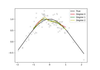
The degree of smoothing functions is controled using the degree parameter. A degree of 0 corresponds to locally constant, a degree of 1 to locally linear and a degree of 2 to locally quadratic, etc. High degrees can cause overfitting.
The implementation is adapted from [3].
- Parameters:
kernel_name (str) – Kernel name used as weight (gaussian, epanechnikov, tricube, bisquare).
bandwidth (float) – Strictly positive. Control the size of the associated neighborhood.
degree (int) – Degree of the local polynomial to fit. If
degree = 0, we fit the local constant estimator (equivalent to the Nadaraya-Watson estimator). Ifdegree = 1, we fit the local linear estimator. Ifdegree = 2, we fit the local quadratic estimator.robust (bool) – Whether to apply the robustification procedure from [1], page 831.
- Attributes:
kernel (Callable) – Function associated to the kernel name.
poly_features (PolynomialFeatures) – An instance of
sklearn.preprocessing.PolynomialFeaturesused to create design matrices. It includes an intercept and interactions for multidimensional inputs.
Notes
This methods is memory-based and thus require no training; all the work is performed at evaluation time [2]. For now, no
fitfunction is necessary and only apredictis implemented.References
Methods
predict(y, x[, x_new])Predict using local polynomial regression.
- predict(y, x, x_new=None)[source]#
Predict using local polynomial regression.
- Parameters:
- Returns:
Return predicted values.
- Return type:
npt.NDArray[np.float64], shape = (n_samples,)
Notes
Be careful that, for two-dimensional and higher-dimensional data, not passing a
x_newargument may result to something unexpected as for now, the functionnp.uniquere-order the columns of the data. To be sure of the results, please provide ax_newargument.Examples
For one-dimensional data.
>>> n_points = 101
>>> x = np.linspace(0, 1, n_points)
>>> y = np.sin(x) + np.random.normal(0, 0.05, n_points)
>>> x_new = np.linspace(0, 1, 11)
>>> lp = LocalPolynomial(
...     kernel_name='epanechnikov', bandwidth=0.3, degree=1
... )
>>> lp.predict(y=y, x=x, x_new=x_new)
For two-dimensional data.
>>> n_points = 51
>>> pts = np.linspace(0, 1, n_points)
>>> xx, yy = np.meshgrid(pts, pts, indexing='ij')
>>> x = np.column_stack([xx.flatten(), yy.flatten()])
>>> eps = np.random.normal(0, 0.1, len(x))
>>> y = np.sin(x[:, 0]) * np.cos(x[:, 1]) + eps
>>> lp = LocalPolynomial(
...     kernel_name='epanechnikov', bandwidth=0.3, degree=2
... )
>>> lp.predict(y=y, x=x, x_new=x_new)
Examples using FDApy.preprocessing.LocalPolynomial#
Smoothing of 1D data using local polynomial regression

Smoothing of 2D data using local polynomial regression