FPCA of 1-dimensional sparse data

Example of functional principal components analysis of 1-dimensional sparse data.

# Author: Steven Golovkine <steven_golovkine@icloud.com>
# License: MIT

# Load packages
import matplotlib.pyplot as plt
import numpy as np

from FDApy.representation import DenseArgvals
from FDApy.simulation import KarhunenLoeve
from FDApy.preprocessing import UFPCA
from FDApy.visualization import plot

# Set general parameters
rng = 42
n_obs = 50

# Parameters of the basis
name = "fourier"
n_functions = 25
argvals = DenseArgvals({"input_dim_0": np.linspace(0, 1, 101)})

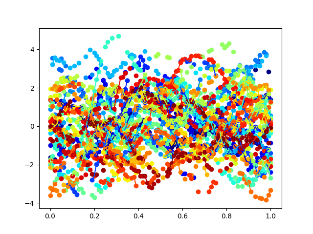
We simulate \(N = 50\) curves on the one-dimensional observation grid \(\{0, 0.01, 0.02, \cdots, 1\}\), based on the first \(K = 25\) Fourier basis functions on \([0, 1]\) and the variance of the scores random variables decreasing exponentially.

kl = KarhunenLoeve(
    n_functions=n_functions, basis_name=name, argvals=argvals, random_state=rng
)
kl.new(n_obs=n_obs, clusters_std="exponential")
kl.add_noise_and_sparsify(noise_variance=0.01, percentage=0.5, epsilon=0.05)
data = kl.sparse_data

_ = plot(data)

Covariance decomposition

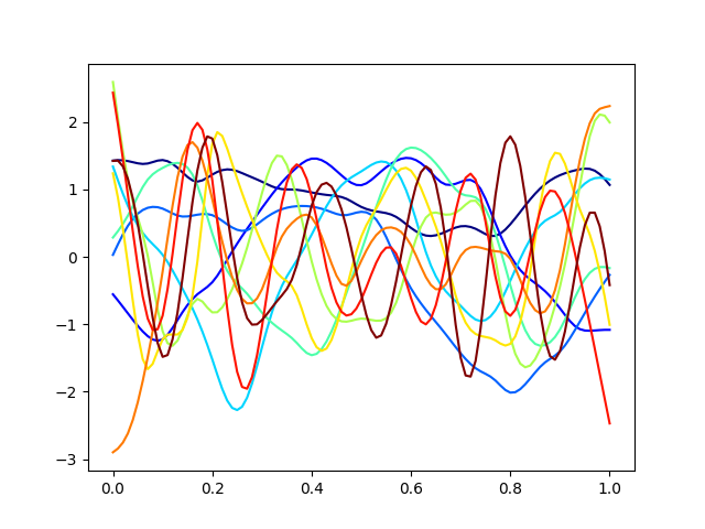
We perform a univariate FPCA with a predefined number of components using a decomposition of the covariance operator.

ufpca_cov = UFPCA(n_components=10, method="covariance")
ufpca_cov.fit(data, method_smoothing="PS")

# Plot the eigenfunctions
_ = plot(ufpca_cov.eigenfunctions)

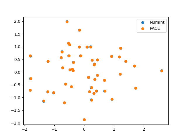
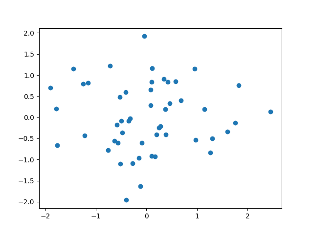
We estimate the scores, which is the projection of the curves onto the eigenfunctions, by numerical integration and using PACE.

scores_numint = ufpca_cov.transform(data, method="NumInt")
scores_pace = ufpca_cov.transform(data, method="PACE")

# Plot of the scores
plt.scatter(scores_numint[:, 0], scores_numint[:, 1], label="NumInt")
plt.scatter(scores_pace[:, 0], scores_pace[:, 1], label="PACE")
plt.legend()
plt.show()

Finally, we reconstruct the curves using the previously computed scores.

data_recons_numint = ufpca_cov.inverse_transform(scores_numint)
data_recons_pace = ufpca_cov.inverse_transform(scores_pace)

Inner-product matrix decomposition

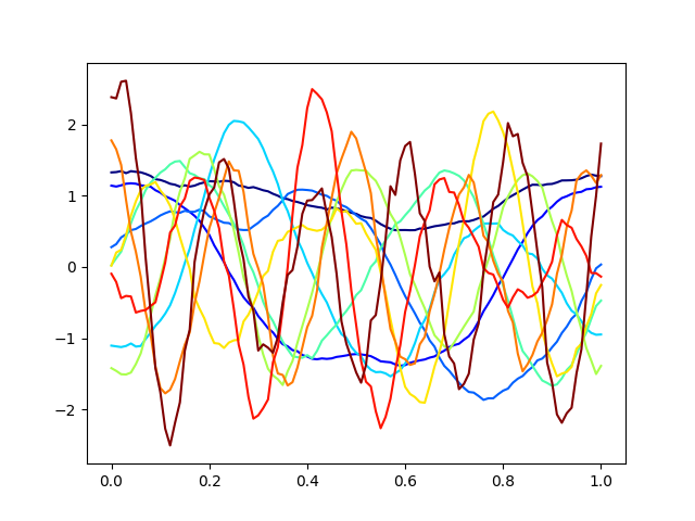
Now, we perform a univariate FPCA using a decomposition of the inner-product matrix.

ufpca_innpro = UFPCA(n_components=10, method="inner-product")
ufpca_innpro.fit(data, method_smoothing="PS")

# Plot the eigenfunctions
_ = plot(ufpca_innpro.eigenfunctions)
plt.show()

As previously, we estimate the scores, but we use the eigenvectors from the decomposition of the inner-product matrix. Note that, here, we do not pass a dataset as argument of the transform method.

scores_innpro = ufpca_innpro.transform(method="InnPro")

# Plot of the scores
_ = plt.scatter(scores_innpro[:, 0], scores_innpro[:, 1])

Finally, we reconstruct the curves using the scores.

data_recons_innpro = ufpca_innpro.inverse_transform(scores_innpro)

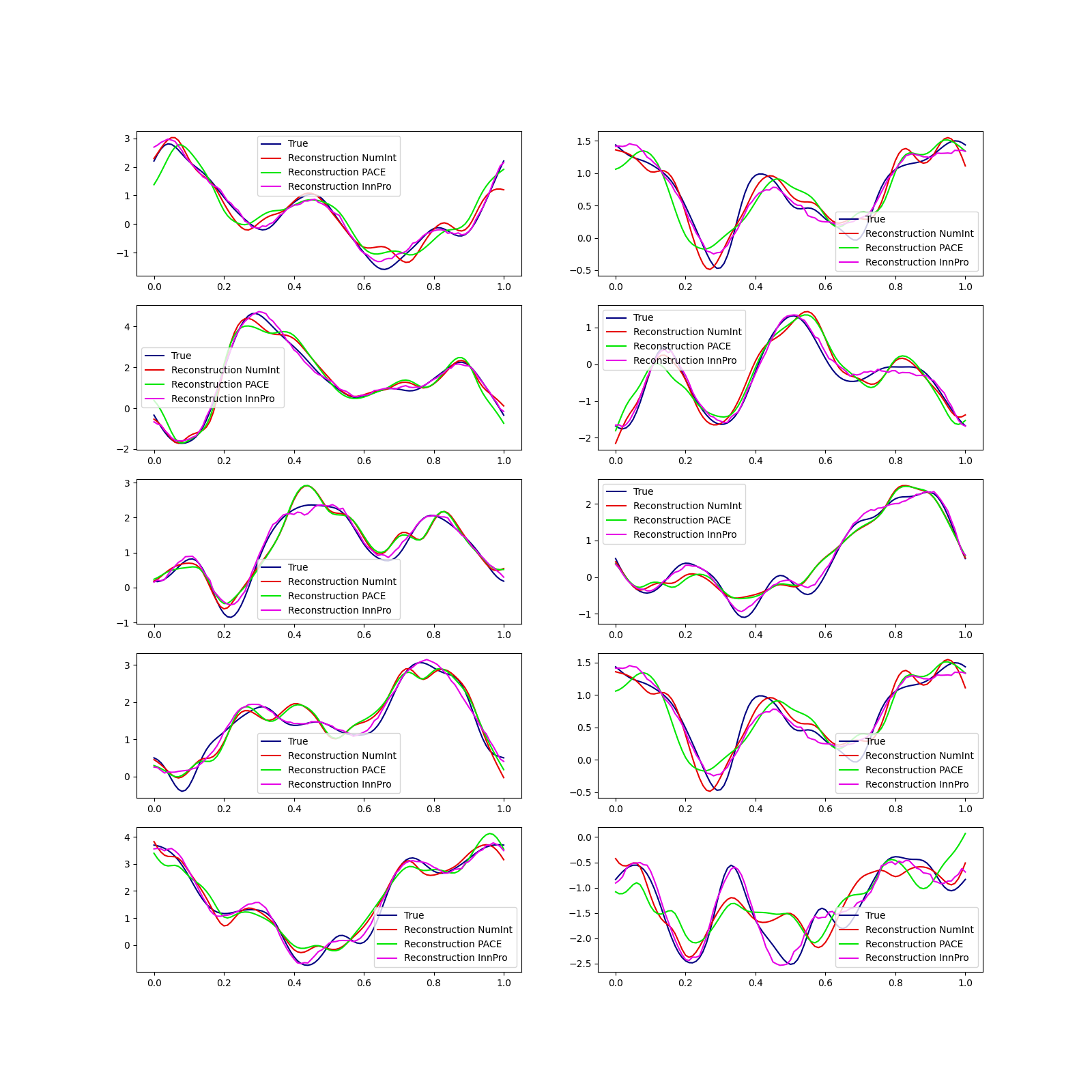
Comparison of the methods

We visually compare the methods by plotting a sample of curves and their reconstruction.

colors_numint = np.array([[0.9, 0, 0, 1]])
colors_pace = np.array([[0, 0.9, 0, 1]])
colors_innpro = np.array([[0.9, 0, 0.9, 1]])

fig, axes = plt.subplots(nrows=5, ncols=2, figsize=(16, 16))
for idx_plot, idx in enumerate(np.random.choice(n_obs, 10)):
    temp_ax = axes.flatten()[idx_plot]
    temp_ax = plot(kl.data[idx], ax=temp_ax, label="True")
    plot(
        data_recons_numint[idx],
        colors=colors_numint,
        ax=temp_ax,
        label="Reconstruction NumInt",
    )
    plot(
        data_recons_pace[idx],
        colors=colors_pace,
        ax=temp_ax,
        label="Reconstruction PACE",
    )
    plot(
        data_recons_innpro[idx],
        colors=colors_innpro,
        ax=temp_ax,
        label="Reconstruction InnPro",
    )
    temp_ax.legend()
plt.show()