FPCA of 2-dimensional data

Example of functional principal components analysis of 2-dimensional data.

# Author: Steven Golovkine <steven_golovkine@icloud.com>
# License: MIT

# Load packages
import matplotlib.pyplot as plt
import numpy as np

from FDApy.simulation.karhunen import KarhunenLoeve
from FDApy.preprocessing.dim_reduction.fpca import UFPCA
from FDApy.preprocessing.dim_reduction.fcp_tpa import FCPTPA
from FDApy.visualization.plot import plot


# Set general parameters
rng = 42
n_obs = 50

# Parameters of the basis
name = 'fourier'
n_functions = 5
argvals = np.linspace(0, 1, 21)

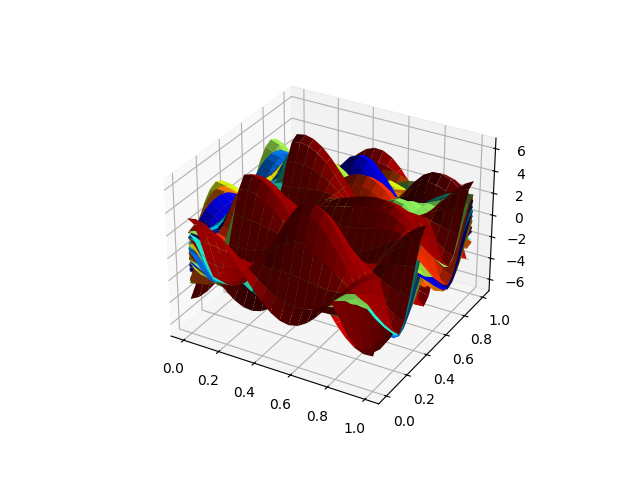
We simulate \(N = 50\) images on the two-dimensional observation grid \(\{0, 0.05, 0.1, \cdots, 1\} \times \{0, 0.05, 0.1, \cdots, 1\}\), based on the tensor product of the first \(K = 5\) Fourier basis functions on \([0, 1] \times [0, 1]\) and the variance of the scores random variables decreases exponentially.

kl = KarhunenLoeve(
    basis_name=name, n_functions=n_functions, argvals=argvals,
    dimension='2D', add_intercept=False, random_state=rng
)
kl.new(n_obs=n_obs, clusters_std='exponential')
data = kl.data

_ = plot(data)

FCP-TPA decomposition

# Hyperparameters for FCP-TPA
n_points = data.n_points
mat_v = np.diff(np.identity(n_points[0]))
mat_w = np.diff(np.identity(n_points[1]))

penal_v = np.dot(mat_v, mat_v.T)
penal_w = np.dot(mat_w, mat_w.T)

ufpca_fcptpa = FCPTPA(n_components=5, normalize=True)
ufpca_fcptpa.fit(
    data,
    penalty_matrices={'v': penal_v, 'w': penal_w},
    alpha_range={'v': (1e-4, 1e4), 'w': (1e-4, 1e4)},
    tolerance=1e-4,
    max_iteration=15,
    adapt_tolerance=True
)

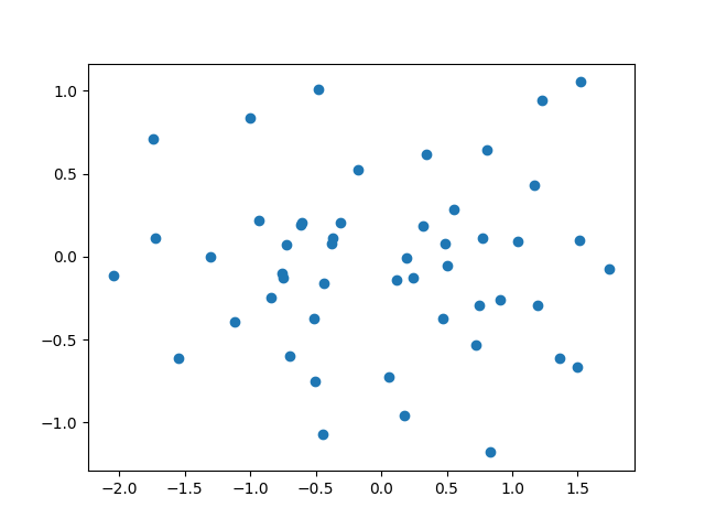
We estimate the scores.

scores_fcptpa = ufpca_fcptpa.transform(data)

# Plot of the scores
_ = plt.scatter(scores_fcptpa[:, 0], scores_fcptpa[:, 1])

# Reconstruct the curves using the scores.
data_recons_fcptpa = ufpca_fcptpa.inverse_transform(scores_fcptpa)

Inner-product matrix decomposition

Perform univariate FPCA using a decomposition of the inner-product matrix.

ufpca_innpro = UFPCA(n_components=5, method='inner-product')
ufpca_innpro.fit(data)

/home/docs/checkouts/readthedocs.org/user_builds/fdapy/checkouts/v1.0.0/FDApy/preprocessing/dim_reduction/fpca.py:786: UserWarning: The estimation of the covariance is not performed for 2-dimensional data.
  warnings.warn((

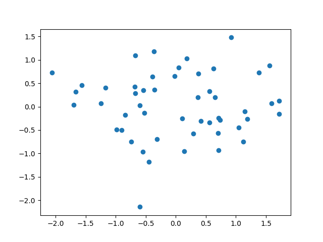
Estimate the scores – projection of the curves onto the eigenfunctions – using the eigenvectors from the decomposition of the inner-product matrix. numerical integration.

scores_innpro = ufpca_innpro.transform(method='InnPro')

# Plot of the scores
_ = plt.scatter(scores_innpro[:, 0], scores_innpro[:, 1])

Reconstruct the curves using the scores.

data_recons_innpro = ufpca_innpro.inverse_transform(scores_innpro)

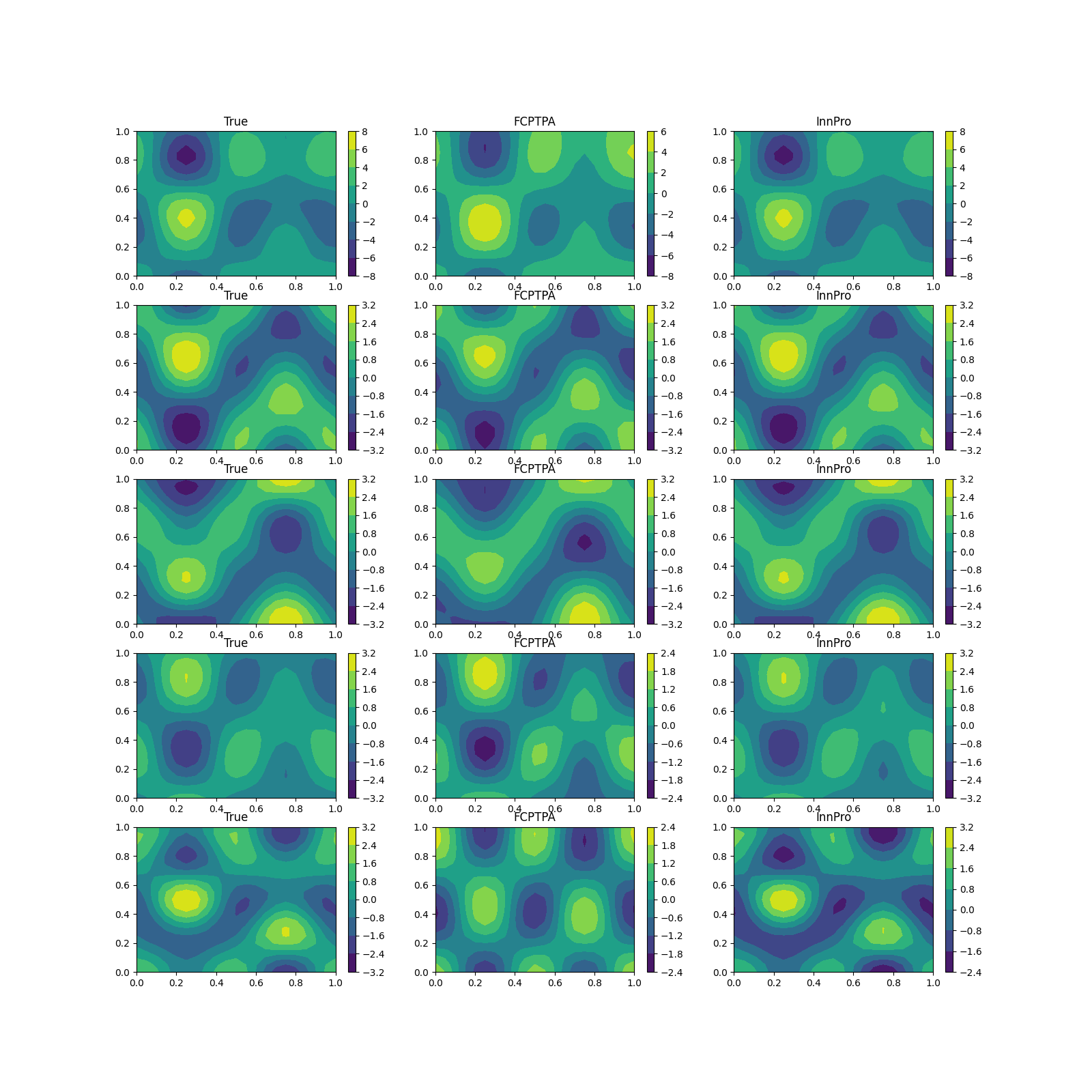
Plot an example of the curve reconstruction

fig, axes = plt.subplots(nrows=5, ncols=3, figsize=(16,16))
for idx_plot, idx in enumerate(np.random.choice(n_obs, 5)):
    axes[idx_plot, 0] = plot(data[idx], ax=axes[idx_plot, 0])
    axes[idx_plot, 0].set_title('True')

    axes[idx_plot, 1] = plot(data_recons_fcptpa[idx], ax=axes[idx_plot, 1])
    axes[idx_plot, 1].set_title('FCPTPA')

    axes[idx_plot, 2] = plot(data_recons_innpro[idx], ax=axes[idx_plot, 2])
    axes[idx_plot, 2].set_title('InnPro')
plt.show()