Smoothing of 2D data using P-Splines

Examples of smoothing of two-dimensional data using P-Splines.

Author: Steven Golovkine <steven_golovkine@icloud.com> License: MIT

# Load packages
import matplotlib.pyplot as plt
import numpy as np

from FDApy.preprocessing.smoothing.psplines import PSplines

# Set general parameters
rng = 42
runif = np.random.default_rng(rng).uniform
n_points = 21
n_points_new = 51

# Simulate data
x = np.sort(runif(-1, 1, n_points))
y = np.sort(runif(-1, 1, n_points))
X, Y = np.meshgrid(x, y)
Z = (
    -1 * np.sin(X)
    + 0.5 * np.cos(Y)
    + 0.2 * np.random.normal(loc=0, scale=1, size=X.shape)
)

argvals = [x, y]
Z_vec = Z.ravel()

x_new = np.linspace(-1, 1, n_points_new)
y_new = np.linspace(-1, 1, n_points_new)
X_new, Y_new = np.meshgrid(x_new, y_new)
argvals_new = [x_new, y_new]

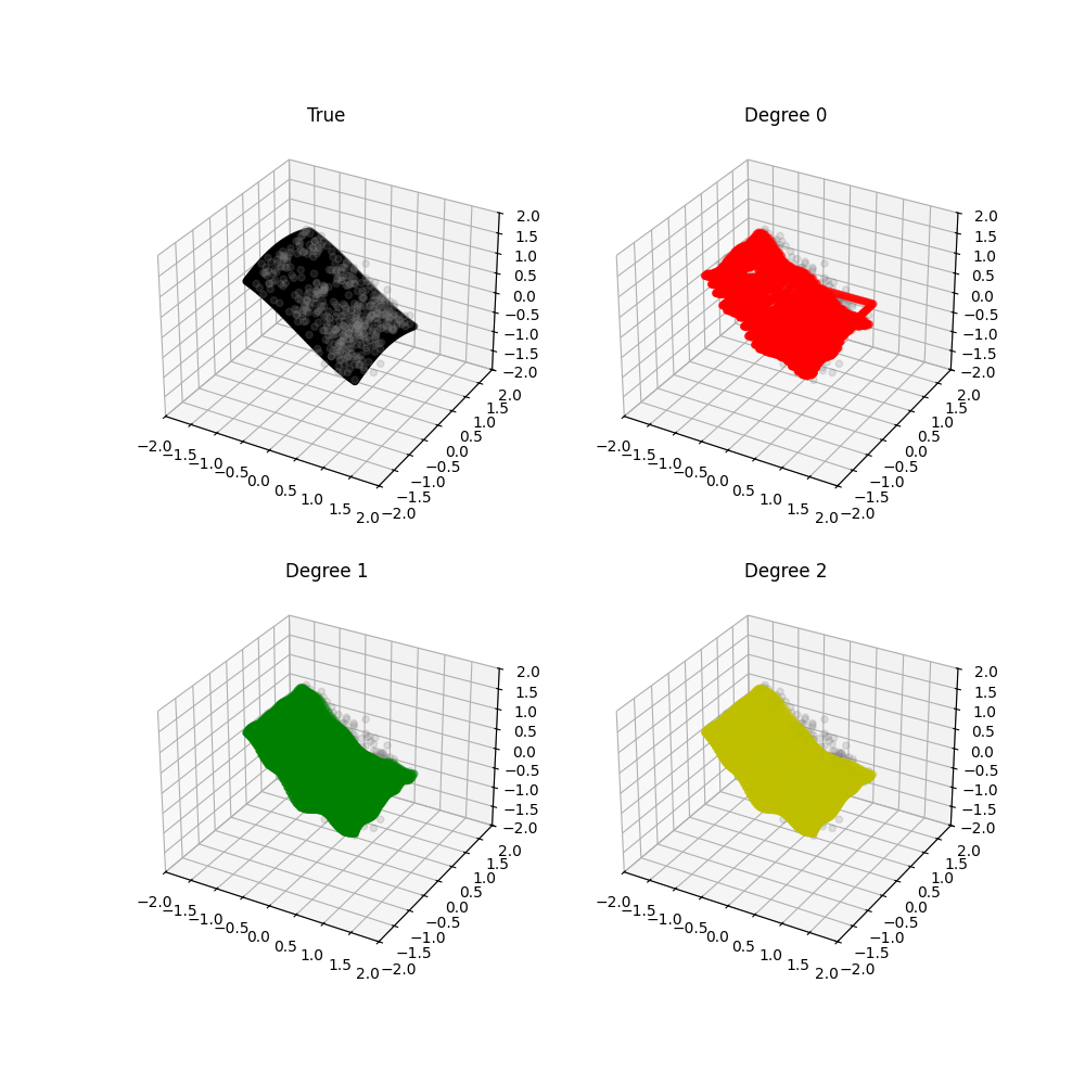
Assess the influence of the degree of the B-Splines basis.

# Fit P-Splines regression with degree 0
ps = PSplines(n_segments=20, degree=0)
ps.fit(Z, argvals, penalty=(1, 1))
y_pred_0 = ps.predict(argvals_new)

# Fit P-Splines regression with degree 1
ps = PSplines(n_segments=20, degree=1)
ps.fit(Z, argvals, penalty=(1, 1))
y_pred_1 = ps.predict(argvals_new)

# Fit P-Splines regression with degree 2
ps = PSplines(n_segments=20, degree=2)
ps.fit(Z, argvals, penalty=(1, 1))
y_pred_2 = ps.predict(argvals_new)

fig = plt.figure(figsize=(10, 10))
# True
ax1 = fig.add_subplot(2, 2, 1, projection="3d")
ax1.set_title("True")
ax1.scatter(X, Y, Z, c="grey", alpha=0.2)
ax1.scatter(X_new, Y_new, -1 * np.sin(X_new) + 0.5 * np.cos(Y_new), c="k")
ax1.set_xlim((-2, 2))
ax1.set_ylim((-2, 2))
ax1.set_zlim((-2, 2))
# Degree 0
ax2 = fig.add_subplot(2, 2, 2, projection="3d")
ax2.set_title("Degree 0")
ax2.scatter(X, Y, Z, c="grey", alpha=0.2)
ax2.scatter(X_new, Y_new, y_pred_0, c="r")
ax2.set_xlim((-2, 2))
ax2.set_ylim((-2, 2))
ax2.set_zlim((-2, 2))
# Degree 1
ax3 = fig.add_subplot(2, 2, 3, projection="3d")
ax3.set_title("Degree 1")
ax3.scatter(X, Y, Z, c="grey", alpha=0.2)
ax3.scatter(X_new, Y_new, y_pred_1, c="g")
ax3.set_xlim((-2, 2))
ax3.set_ylim((-2, 2))
ax3.set_zlim((-2, 2))
# Degree 2
ax4 = fig.add_subplot(2, 2, 4, projection="3d")
ax4.set_title("Degree 2")
ax4.scatter(X, Y, Z, c="grey", alpha=0.2)
ax4.scatter(X_new, Y_new, y_pred_2, c="y")
ax4.set_xlim((-2, 2))
ax4.set_ylim((-2, 2))
ax4.set_zlim((-2, 2))
plt.show()

Assess the influence of the penalty $lambda$.

# Fit P-Splines regression with penalty=10
ps = PSplines(n_segments=20, degree=2)
ps.fit(Z, argvals, penalty=(10, 10))
y_pred_0 = ps.predict(argvals_new)

# Fit P-Splines regression with penalty=1
ps = PSplines(n_segments=20, degree=2)
ps.fit(Z, argvals, penalty=(1, 1))
y_pred_1 = ps.predict(argvals_new)

# Fit P-Splines regression with penalty=0.1
ps = PSplines(n_segments=20, degree=2)
ps.fit(Z, argvals, penalty=(0.1, 0.1))
y_pred_2 = ps.predict(argvals_new)

fig = plt.figure(figsize=(10, 10))
# True
ax1 = fig.add_subplot(2, 2, 1, projection="3d")
ax1.set_title("True")
ax1.scatter(X, Y, Z, c="grey", alpha=0.2)
ax1.scatter(X_new, Y_new, -1 * np.sin(X_new) + 0.5 * np.cos(Y_new), c="k")
ax1.set_xlim((-2, 2))
ax1.set_ylim((-2, 2))
ax1.set_zlim((-2, 2))
# Degree 0
ax2 = fig.add_subplot(2, 2, 2, projection="3d")
ax2.set_title("$\lambda = 10$")
ax2.scatter(X, Y, Z, c="grey", alpha=0.2)
ax2.scatter(X_new, Y_new, y_pred_0, c="r")
ax2.set_xlim((-2, 2))
ax2.set_ylim((-2, 2))
ax2.set_zlim((-2, 2))
# Degree 1
ax3 = fig.add_subplot(2, 2, 3, projection="3d")
ax3.set_title("$\lambda = 1$")
ax3.scatter(X, Y, Z, c="grey", alpha=0.2)
ax3.scatter(X_new, Y_new, y_pred_1, c="g")
ax3.set_xlim((-2, 2))
ax3.set_ylim((-2, 2))
ax3.set_zlim((-2, 2))
# Degree 2
ax4 = fig.add_subplot(2, 2, 4, projection="3d")
ax4.set_title("$\lambda = 0.1$")
ax4.scatter(X, Y, Z, c="grey", alpha=0.2)
ax4.scatter(X_new, Y_new, y_pred_2, c="y")
ax4.set_xlim((-2, 2))
ax4.set_ylim((-2, 2))
ax4.set_zlim((-2, 2))
plt.show()