Simulation of clusters of multivariate functional data

Examples of simulation of clusters of multivariate functional data.

# Author: Steven Golovkine <steven_golovkine@icloud.com>
# License: MIT

# Load packages
import numpy as np

from FDApy.representation import DenseArgvals
from FDApy.simulation import KarhunenLoeve
from FDApy.visualization import plot_multivariate

# Set general parameters
rng = 42
n_obs = 20

# Define the random state
random_state = np.random.default_rng(rng)

# Parameters of the basis
name = ["fourier", "wiener"]
n_functions = [5, 5]
argvals = [
    DenseArgvals({"input_dim_0": np.linspace(0, 1, 101)}),
    DenseArgvals({"input_dim_0": np.linspace(0, 1, 101)}),
]

# Parameters of the clusters
n_clusters = 2
mean = np.array([0, 0])
covariance = np.array([[1, -0.6], [-0.6, 1]])
centers = random_state.multivariate_normal(mean, covariance, size=n_functions[0])

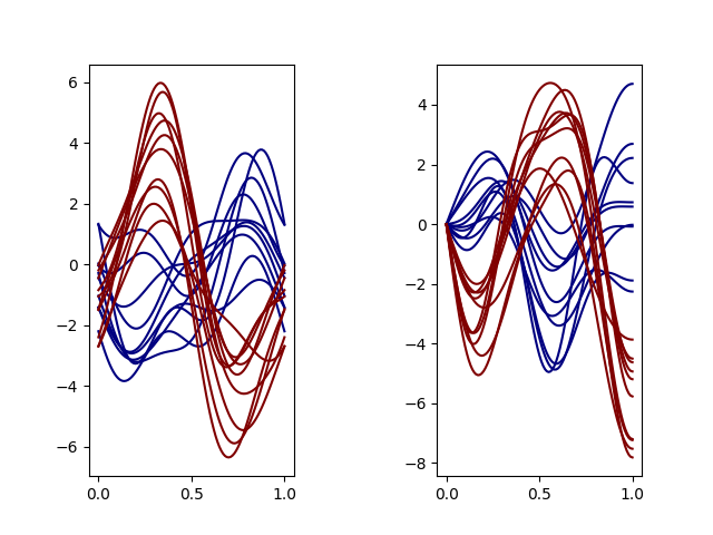
First example — We simulate \(N = 20\) curves of a 2-dimensional process. The first component of the process is defined on the one-dimensional observation grid \(\{0, 0.01, 0.02, \cdots, 1\}\), based on the first \(K = 5\) Fourier basis functions on \([0, 1]\) and the decreasing of the variance of the scores is exponential. The second component of the process is defined on the one-dimensional observation grid \(\{0, 0.01, 0.02, \cdots, 1\}\), based on the first \(K = 5\) Wiener basis functions on \([0, 1]\) and the decreasing of the variance of the scores is exponential. The clusters are defined through the coefficients in the Karhunen-Loève decomposition. The centers of the clusters are generated as Gaussian random variables with parameters defined by mean and covariance.

kl = KarhunenLoeve(
    basis_name=name, argvals=argvals, n_functions=n_functions, random_state=rng
)
kl.new(n_obs=n_obs, n_clusters=n_clusters, centers=centers, clusters_std="exponential")

_ = plot_multivariate(kl.data, kl.labels)

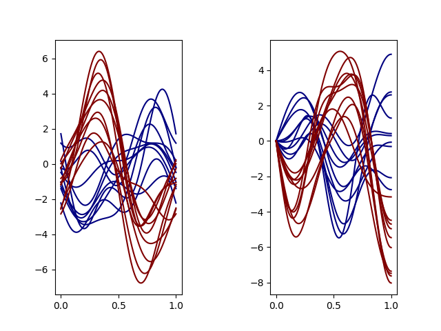
Second example — We simulate \(N = 20\) curves of a 2-dimensional process. The first component of the process is defined on the one-dimensional observation grid \(\{0, 0.01, 0.02, \cdots, 1\}\), based on the first \(K = 5\) Fourier basis functions on \([0, 1]\) and the decreasing of the variance of the scores is linear. The second component of the process is defined on the one-dimensional observation grid \(\{0, 0.01, 0.02, \cdots, 1\}\), based on the first \(K = 5\) Wiener basis functions on \([0, 1]\) and the decreasing of the variance of the scores is linear. The clusters are defined through the coefficients in the Karhunen-Loève decomposition. The centers of the clusters are generated as Gaussian random variables with parameters defined by mean and covariance.

kl = KarhunenLoeve(
    basis_name=name, argvals=argvals, n_functions=n_functions, random_state=rng
)
kl.new(n_obs=n_obs, n_clusters=n_clusters, centers=centers, clusters_std="linear")

_ = plot_multivariate(kl.data, kl.labels)