Representation of univariate and irregular functional data

Examples of representation of univariate and irregular functional data.

# Author: Steven Golovkine <steven_golovkine@icloud.com>
# License: MIT

# Load packages
import numpy as np

from FDApy import IrregularFunctionalData
from FDApy.representation import DenseArgvals, IrregularArgvals, IrregularValues
from FDApy.visualization import plot

The representation of irregular functional data

We are showing the building blocks of the representation of univariate and irregular functional data. To define a FunctionalData object, we need a set of argvals (the sampling points of the curves) and a set of values (the observed points of the curves). The sampling points of the data are defined as a dictionary where each entry is another dictionary that represents an input dimension (one entry corresponds to curves, two entries correspond to surface, …). Each entry of the dictionary corresponds to the sampling points of one observation. The values of the functional data are defined in a dictionary where each entry represents an observation as an npt.NDArray. Each entry should have the same dimension has the corresponding entry in the argvals dictionary.

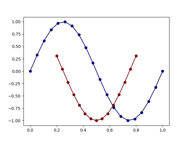
For unidimensional functional data

First, we will define unidimensional functional data. We consider twenty sampling points for the first observations and fifteen sampling points for the second observations.

argvals = IrregularArgvals(
    {
        0: DenseArgvals({"input_dim_0": np.linspace(0, 1, num=20)}),
        1: DenseArgvals({"input_dim_0": np.linspace(0.2, 0.8, num=15)}),
    }
)
X = IrregularValues(
    {
        0: np.sin(2 * np.pi * argvals[0]["input_dim_0"]),
        1: np.cos(2 * np.pi * argvals[1]["input_dim_0"]),
    }
)

fdata = IrregularFunctionalData(argvals=argvals, values=X)

_ = plot(fdata)

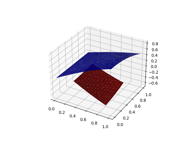
For two-dimensional functional data

Second, we will defined two-dimensional functional data. We consider a grid of \(20 \times 20\) sampling points for the first observation and a grid of \(15 \times 15\) sampling points for the second observation.

argvals = IrregularArgvals(
    {
        0: DenseArgvals(
            {
                "input_dim_0": np.linspace(0, 1, num=20),
                "input_dim_1": np.linspace(0, 1, num=20),
            }
        ),
        1: DenseArgvals(
            {
                "input_dim_0": np.linspace(0.2, 0.8, num=15),
                "input_dim_1": np.linspace(0.2, 0.8, num=15),
            }
        ),
    }
)
X = IrregularValues(
    {
        0: np.outer(
            np.sin(argvals[0]["input_dim_0"]), np.cos(argvals[0]["input_dim_1"])
        ),
        1: np.outer(
            np.sin(-argvals[1]["input_dim_0"]), np.cos(argvals[1]["input_dim_1"])
        ),
    }
)

fdata = IrregularFunctionalData(argvals=argvals, values=X)

_ = plot(fdata)