Simulation of functional data

Examples of simulation of functional data and the effect of adding noise and sparsification.

# Author: Steven Golovkine <steven_golovkine@icloud.com>
# License: MIT

# Load packages
from FDApy.simulation import KarhunenLoeve
from FDApy.visualization import plot

# Set general parameters
rng = 42
n_obs = 10

# Parameters of the basis
name = 'bsplines'
n_functions = 5

For one dimensional data

We simulate \(N = 10\) curves on the one-dimensional observation grid \(\{0, 0.01, 0.02, \cdots, 1\}\), based on the first \(K = 5\) B-splines basis functions on \([0, 1]\) and the variance of the scores random variables equal to \(1\).

kl = KarhunenLoeve(
    basis_name=name, n_functions=n_functions, random_state=rng
)
kl.new(n_obs=n_obs)

_ = plot(kl.data)

Adding noise — We can generates a noisy version of the functional data by adding i.i.d. realizations of the random variable \(\varepsilon \sim \mathcal{N}(0, \sigma^2)\) to the observation. In this example, we set \(\sigma^2 = 0.05\).

# Add some noise to the simulation.
kl.add_noise(0.05)

# Plot the noisy simulations
_ = plot(kl.noisy_data)

Sparsification — We can generates a sparsified version of the functional data object by randomly removing a certain percentage of the sampling points. The percentage of retain samplings points can be supplied by the user. In this example, the retained number of observations will be different for each curve and be randomly drawn between \(0.45\) and \(0.55\).

# Sparsify the data
kl.sparsify(percentage=0.5, epsilon=0.05)

_ = plot(kl.sparse_data)

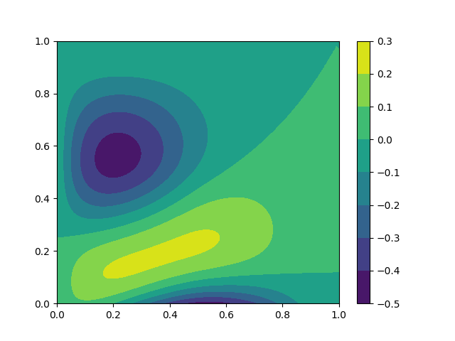
For two dimensional data

We simulate \(N = 1\) image on the two-dimensional observation grid \(\{0, 0.01, 0.02, \cdots, 1\} \times \{0, 0.01, 0.02, \cdots, 1\}\), based on the tensor product of the first \(K = 25\) B-splines basis functions on \([0, 1] \times [0, 1]\) and the variance of the scores random variables equal to \(1\).

kl = KarhunenLoeve(
    basis_name=name, dimension='2D', n_functions=n_functions, random_state=rng
)
kl.new(n_obs=1)

_ = plot(kl.data)

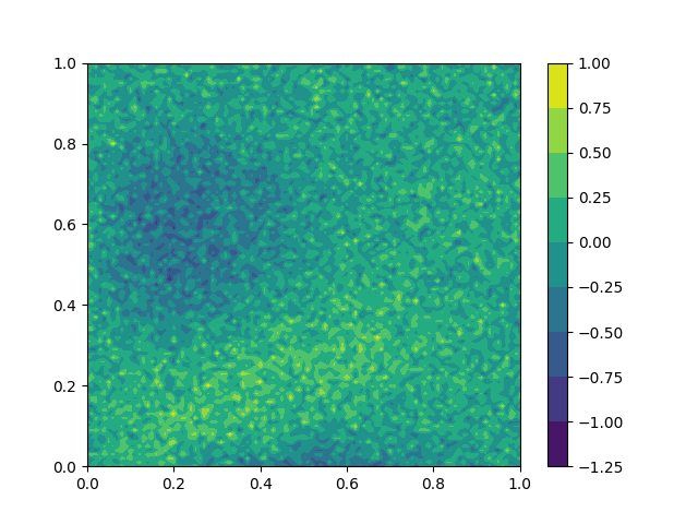
Adding noise — We can generates a noisy version of the functional data by adding i.i.d. realizations of the random variable \(\varepsilon \sim \mathcal{N}(0, \sigma^2)\) to the observation. In this example, we set \(\sigma^2 = 0.05\).

# Add some noise to the simulation.
kl.add_noise(0.05)

# Plot the noisy simulations
_ = plot(kl.noisy_data)

Sparsification — The sparsification is not implemented for two-dimensional (and higher) data.