Canadian weather dataset

Example of the Canadian weather dataset.

# Author: Steven Golovkine <steven_golovkine@icloud.com>
# License: MIT

# Load packages
import matplotlib.pyplot as plt
import numpy as np

from FDApy.representation.argvals import DenseArgvals
from FDApy.preprocessing.dim_reduction.fpca import UFPCA

from FDApy.misc.loader import read_csv
from FDApy.visualization.plot import plot

# Load data
temp_data = read_csv('../data/canadian_temperature_daily.csv', index_col=0)


_ = plot(temp_data)

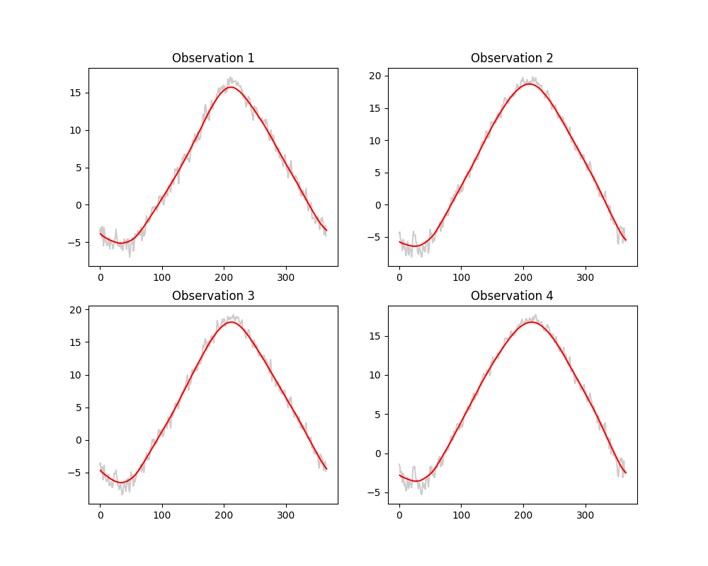
Smooth the data

points = DenseArgvals({'input_dim_0': np.linspace(1, 365, 365)})
kernel_name = "epanechnikov"
bandwidth = 30
degree = 1

temp_smooth = temp_data.smooth(
    points=points, kernel_name=kernel_name, bandwidth=bandwidth, degree=degree
)


fig, axes = plt.subplots(2, 2, figsize=(10, 8))
for idx, ax in enumerate(axes.flat):
    plot(temp_data[idx], colors='k', alpha=0.2, ax=ax)
    plot(temp_smooth[idx], colors='r', ax=ax)
    ax.set_title(f"Observation {idx + 1}")
plt.show()

Perform UFPCA

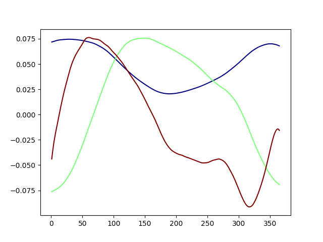
ufpca = UFPCA(n_components=0.99, method='inner-product')
ufpca.fit(temp_smooth)

# Plot the eigenfunctions
_ = plot(ufpca.eigenfunctions)

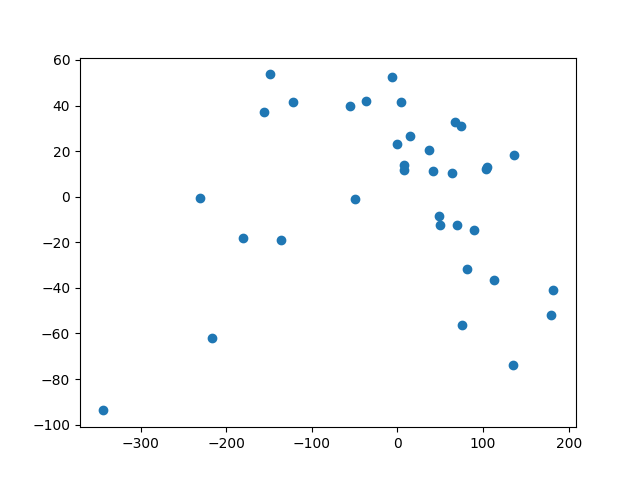
Compute the scores

scores = ufpca.transform(method='InnPro')

# Plot of the scores
_ = plt.scatter(scores[:, 0], scores[:, 1])

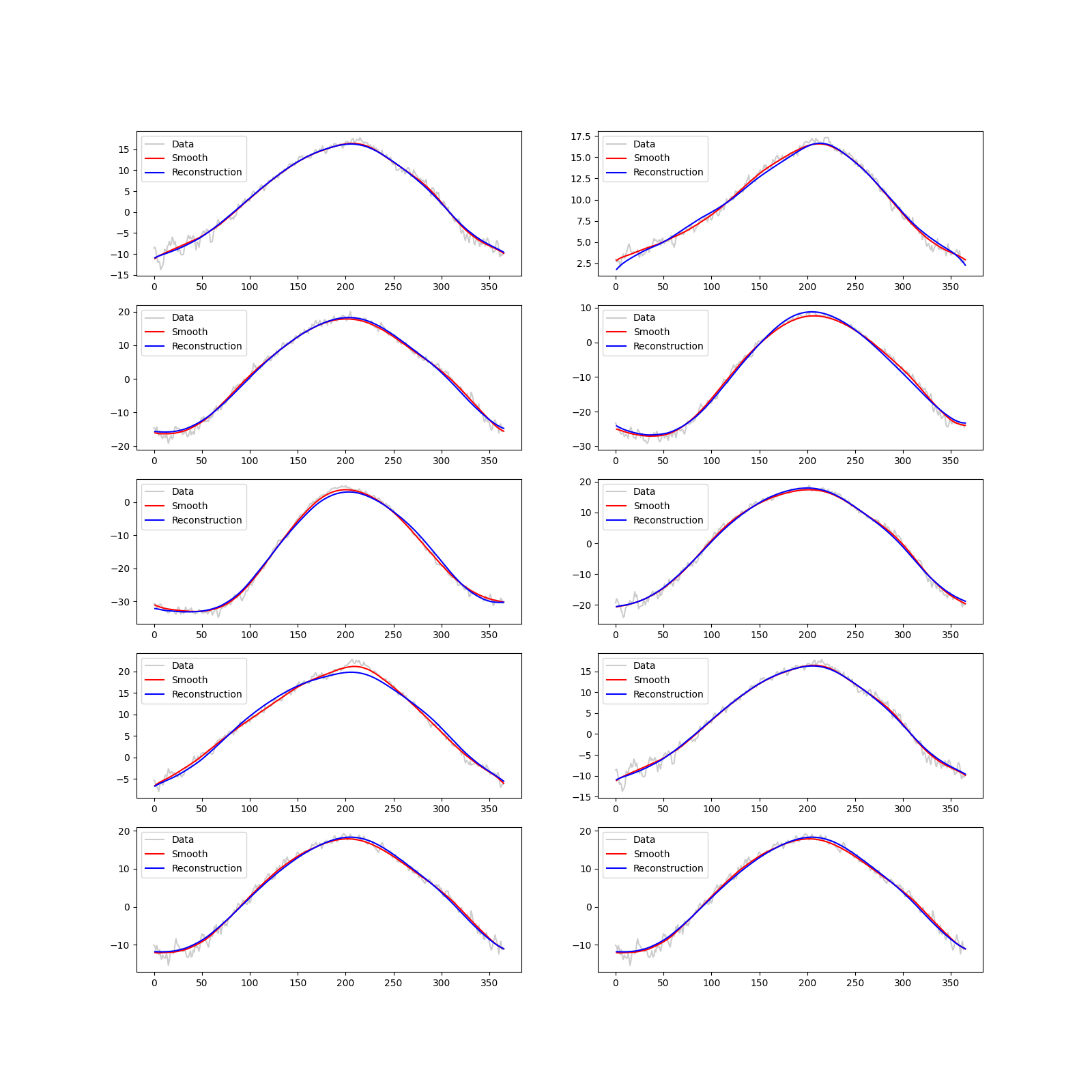
Reconstruction of the curves

data_recons = ufpca.inverse_transform(scores)

Plot of the reconstruction

fig, axes = plt.subplots(nrows=5, ncols=2, figsize=(16,16))
for idx_plot, idx in enumerate(np.random.choice(temp_data.n_obs, 10)):
    temp_ax = axes.flatten()[idx_plot]
    temp_ax = plot(temp_data[idx], colors='k', alpha=0.2, ax=temp_ax, label='Data')
    plot(temp_smooth[idx], colors='r', ax=temp_ax, label='Smooth')
    plot(data_recons[idx], colors='b', ax=temp_ax, label='Reconstruction')
    temp_ax.legend()
plt.show()