Multivariate Basis of multi-dimensional data

# Author: Steven Golovkine <steven_golovkine@icloud.com>
# License: MIT

# Load packages
import numpy as np
import matplotlib.pyplot as plt

from FDApy.representation.basis import MultivariateBasis
from FDApy.visualization.plot import plot

# Parameters
n_components = 2
basis_name = 'fourier'
argvals = [
    np.linspace(0, 1, 11),
    np.linspace(0, 0.5, 11)
]
n_functions = 3
dimension = ['1D', '2D']
random_state = np.random.default_rng(42)

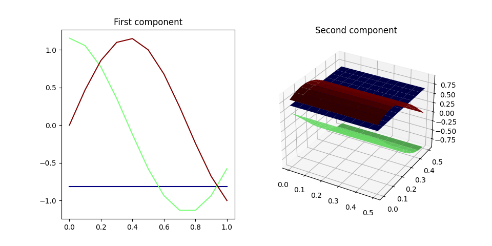
Using split

basis = MultivariateBasis(
    simulation_type='split',
    n_components=n_components,
    name=basis_name,
    n_functions=n_functions,
    dimension=dimension,
    argvals=argvals,
    norm=False,
    rchoice=random_state.choice
)

# Plot of the basis
fig = plt.figure(figsize=plt.figaspect(0.5))

ax = fig.add_subplot(1, 2, 1)
ax = plot(basis.data[0], ax=ax)
ax.set_title('First component')

ax = fig.add_subplot(1, 2, 2, projection='3d')
ax = plot(basis.data[1], ax=ax)
ax.set_title('Second component')

plt.show()

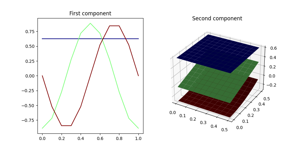
Using weighted

basis = MultivariateBasis(
    simulation_type='weighted',
    n_components=n_components,
    name=['fourier', 'legendre'],
    n_functions=n_functions,
    dimension=dimension,
    argvals=argvals,
    norm=False,
    runif=random_state.uniform
)

# Plot of the basis
fig = plt.figure(figsize=plt.figaspect(0.5))

ax = fig.add_subplot(1, 2, 1)
ax = plot(basis.data[0], ax=ax)
ax.set_title('First component')

ax = fig.add_subplot(1, 2, 2, projection='3d')
ax = plot(basis.data[1], ax=ax)
ax.set_title('Second component')

plt.show()